


Resolution
Authors: Gregory Hollows, Nicholas James
This is Section 2.2 of the Imaging Resource Guide.
Resolution is an imaging system’s ability to reproduce object detail. It can be influenced by factors such as the type of lighting used, the sensor pixel size, and the capabilities of the optics. The smaller the object detail, the higher the required resolution.
Dividing the number of horizontal or vertical pixels on a sensor into the size of the object one wishes to observe will indicate how much space each pixel covers on the object and can be used to estimate resolution. However, this does not truly determine if the information on the pixel is distinguishable from the information on any other pixel.
It is important to understand what can limit system resolution. Figure 1 shows a pair of squares on a white background. If the squares are imaged onto neighboring pixels on the camera sensor, they will appear to be one larger rectangle (a), rather than two separate squares (b). To distinguish the squares, at least one pixel must be between them. This minimum distance is the limiting resolution of the system. The absolute limitation is defined by the size of the pixels on the sensor and number of pixels on the sensor.

Figure 1: Resolving two squares. If the space between the squares is too small (a) the camera sensor will be unable to resolve them as separate objects.
The Line Pair and Sensor Limitations
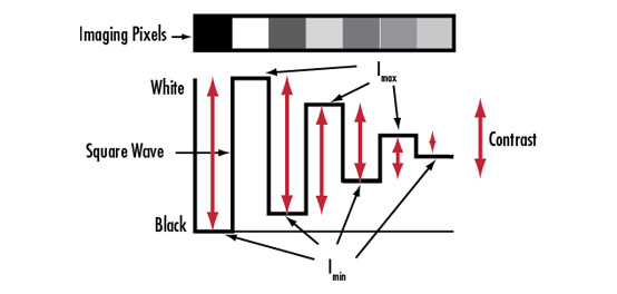
Resolution is often reported as a dimension. This concept of resolution being a minimum size that is resolvable by a lens or system is not a complete description of resolution. Resolution is more accurately described as a frequency, measured in line pairs per millimeter $ \left[ \small{\tfrac{\text{lp}}{\text{mm}}} \right] $. A line pair is a pair of black and white squares in object space. Lens resolution is unfortunately not absolute. At a given resolution, the ability to see the two squares as separate entities will be dependent on greyscale level. A system can more easily resolve a line pair if the difference in the greyscales of the squares and space between them is greater (Figure 1b). This greyscale difference is known as contrast. Resolution is thus defined as a spatial frequency, given in $ \left[ \small{\tfrac{\text{lp}}{\text{mm}}} \right] $, at which a specific contrast is achieved.
Contrast is set by convention for different lens and camera manufacturers but is usually specified for lenses to be 20%. For this reason, calculating resolution in terms of $ \left[ \small{\tfrac{\text{lp}}{\text{mm}}} \right] $ is extremely useful when comparing lenses and for determining the best choice for given sensors and applications (for more information, read Contrast).
The sensor is where the system resolution calculation begins. By starting with the sensor, it is easier to determine the lens performance required to match the sensor or other application requirements. The highest frequency resolvable by a sensor, the Nyquist frequency, is effectively two pixels or one line pair $ \small{\left( 2 \text{ pixels} = 1 \text{ cycle} = 1 \text{ line pair, or lp} \right)} $. Table 1 shows the Nyquist limit associated with pixel sizes found on some common sensors. The resolution of the sensor $ \left( \xi _{\small{\text{Sensor}}} \right) $, referred to as the system’s image space resolution $ \left( \xi _{\small{\text{Image Space}}} \right) $, is calculated by multiplying the pixel size (s), usually in units of microns, by 2 (to create a pair), and dividing that into 1000 to convert to mm:
Sensors with larger pixels will have lower limiting resolutions. Sensors with smaller pixels will have higher limiting resolutions. How this information is used to determine necessary lens performance can be found in Sensor Performance and Limitations. The limiting resolution on the object to be viewed can be calculated using the relationships between the sensor size, the field of view (FOV), and the number of pixels on the sensor.
Sensor size refers to the size of a camera sensor’s active area, specified by the sensor format size (more information on sensor format can be found in Sensors). However, the exact sensor proportions will vary depending on the aspect ratio, so the nominal sensor formats should be used only as a guideline, especially for telecentric lenses and high magnification objectives. The sensor size (H); horizontal, vertical, or diagonal; can be directly calculated from the pixel size and number of active pixels on the sensor (p).
| Pixel Size (µm) | Associated Nyquist Limit $ \left( \tfrac{\text{lp}}{\text{mm}} \right) $ |
|---|---|
| 1.67 | 299.4 |
| 2.2 | 227.3 |
| 3.45 | 144.9 |
| 4.54 | 110.1 |
| 5.5 | 90.9 |
Table 1: As pixel size increases, the associated Nyquist limit in $ \left[ \small{\tfrac{\text{lp}}{\text{mm}}} \right] $ decreases proportionally.
Object Space Resolution
To determine the absolute minimum resolvable spot viewable on the object, the ratio of the FOV to the sensor size must be calculated. This is also known as the system magnification.
System magnification scales the image space resolution up to the object space resolution $ \left( \xi _{\small{\text{Object Space}}} \right) $.
When developing an application, a system’s object space resolution is typically specified as a length dimension, rather than in $ \left[ \small{\tfrac{\text{lp}}{\text{mm}}} \right] $. There are two ways to make this conversion:
While it is easy to jump to the limiting resolution on the object by using the last formula, it is very useful to determine the imaging space resolution and magnification to simplify lens selection. It is also important to note that there are many additional factors involved, and this limitation is often much lower than what can be easily calculated using the equations. Learn more about contrast limitations and lens selection in Contrast and Types of Machine Vision Lenses.
Resolution and Magnification Example Calculations Using a Sony ICX625 Sensor
Known Parameters:
Pixel Size: 3.45 × 3.45μm
Number of Pixels: 2448 × 2050
Desired FOV (Horizontal): 100mm
Limiting Sensor Resolution:
\begin{align} \xi_{\small{\text{Image Space}}} & = \left( \frac{1}{2 \times s} \right) \times \left( \frac{1000 \large{\unicode[Cambria Math]{x03BC}} \normalsize{\text{m}}}{1 \text{mm}} \right) \\ & = \left( \frac{1}{2 \times 3.45 \large{\unicode[Cambria Math]{x03BC}} \normalsize{\text{m}}} \right) \times \left( \frac{1000 \large{\unicode[Cambria Math]{x03BC}} \normalsize{\text{m}}}{1 \text{mm}} \right) \approx 145 \tfrac{\text{lp}}{ \text{mm}} \end{align}
Sensor Dimensions:
$$ H_{\small{\text{Horizontal}}} = 3.45 \large{\unicode[Cambria Math]{x03BC}} \normalsize{\text{m}} \times 2448 \times \left( \frac{1 \text{mm}}{1000 \large{\unicode[Cambria Math]{x03BC}} \normalsize{\text{m}}} \right) = 8.45 \text{mm} $$
$$ H_{\small{\text{Vertical}}} = 3.45 \large{\unicode[Cambria Math]{x03BC}} \normalsize{\text{m}} \times 2050 \times \left( \frac{1 \text{mm}}{1000 \large{\unicode[Cambria Math]{x03BC}} \normalsize{\text{m}}} \right) = 7.07 \text{mm} $$
Magnification:
$$ m = \frac{8.45 \text{mm}}{100 \text{mm}} = 0.0845X $$
Resolution:
$$ \xi_{\small{\text{Object Space}}} \left[ \large{\unicode[Cambria Math]{x03BC}} \normalsize{\text{m}} \right] = 145 \tfrac{\text{lp}}{\text{mm}} \times 0.0845 = 12.25 \tfrac{\text{lp}}{\text{mm}} \approx 41 \large{\unicode[Cambria Math]{x03BC}} \normalsize{\text{m}} $$


or view regional numbers
QUOTE TOOL
enter stock numbers to begin
Copyright 2023, Edmund Optics Inc., 18 Woodlands Loop #04-00, Singapore 738100
California Consumer Privacy Act (CCPA): Do Not Sell or Share My Personal Information
California Transparency in Supply Chains Act